Decomposing the Move Tree

Locality of Moves

The tablebase is really a multi-dimensional array, one dimension for each piece. The problem is that, whichever way we map this space on the linear array of the tablebase, there will always be some moves that go to positions very far away. Any naive way of generating the tablebase, by running through all lost position sequentially, and generating the 3-ply trees from them to get the predecessor lost positions, will violate the principle of data locality. The consequence of this is that you will constantly need to access data that is not in memory, or not in cache, and thus requires extra disk reads and extra memory loads, slowing you down by orders of magnitude.

To cure this, it is necessary to decompose the task of generating grandparent predecessor lost positions into sub-taks that can be performed with high degree of data locality. Perhaps this is best illustrated on the basis of a simple (and totally unrealistic) example: Suppose you are treating a 1-men EGT with a Rook, and want to follow all Rook moves (e.g. to probe the position after the move) from all Rook positions. No matter in which order you step through the squares, if you generate all moves from a square at at once, (i.e. immediately after one another, without starting from other squares first), you will have to probe positions far away in the sequence of starting squares. E.g. if you scan by rank, by the time you have treated a1-h1, the move targets will have covered all the board, and one of those remaining squares will unavoidably be 56 positions later in the sequence. There simply is no way to try a new square as starting square, without adding many squares to the set of target squares that where reached, but not yet in the sequence of starting squares. So any attempt to order the squares such that those that occurred as target will be used as starting square quickly thereafter is doomed to fail, a your backlog of squares that have to be treated urgently will explode a you go.

However, if you scan the board by rank, and only treat Rook moves along the rank, the task nicely breaks up in groups of 8 squares (forming a rank), and you will never need to access a target square for probing that is removed more than 7 steps in the sequence of starting squares. This sub-task can be performed very efficiently by caching at most 8 positions (1 rank). And it can do it by virtue of the fact that you got rid of the distant probes due to moves along a file, which were causing cache misses of your 8-entry cache, and flushing the nearby entries from it all the time. Of course you would need to treat the Rook moves along the files as well, but this second sub-task could be done while scanning the board file by file, i.e. order the starting squares as a1-a2-a3-... Then again you would only need to cache at most 8 entries (a complete file), on which all probe access would give hits.

The moral lesson is thus that although there is no conceivable order in which you could traverse the EGT that would make all moves or move trees local, it is posible to decompose the task of generating the trees into sub-tasks, for which such a 'scan' order does exist. But this required scan order will be different for all the sub-tasks, which means they cannot be combined into a single scan. Each sub-task will require a separate pass through the EGT, ordering the entries it starts working from in a sequence that suits it best.

Black and White sub-cycles

One way to decompose the retrograde tree is by level. First you do a pass through the EGT treating all white moves from lost(N) positions, generating new won positions. Then you do a second pass, treating all black moves from these new won positions, to get the lost(N+1). Each pass is done with a nesting of the scan loops (for each piece) that scans the pieces that are moved in the inner-most loops, and the pieces of the other color in the outermost loop. This way, you only have to load each entry twice for each full cycle, instead of an undetermined number of times related to the number of moves you have. Drawback is that you have to be able to distinguish won positions found in the previous (white) pass from won positions found earlier. This requires information on the wtm positions beyond the single won-bit. We will refer to this info as the 'newly-won' set. Usually it is a sparse set, so the situation is bearable.

Root Splitting

With root splitting, the tree is subdivided into sub-trees that start with different white moves, but at the next levels do treat all black moves. This requires a working set at least as large as that for the black pass when we split in white and black sub-cycles, and thus seems to offer little advantage. Even if we split the white moves into two groups, we would require two passes through the EGT, just like with splitting in blck and white sub-cycles. And we would have to cache slices that do not only contain all constellations of black pieces, but some of the white pieces on top of it. If the cache (fast storage) is big enough to handle this, though, the advantage is that we do not have to remember between one sub-cycle and the other which of the won positions are newly discovered ones, as we immediately continue with the black levels of the tree if they were, and abort the tree branch if they weren't. Plus, a we shal see below, there is a trick to reduce the number of required accesses by one, which means a 50% reduction if there were only two!

Leapfrog The basic idea of leapfrog is to decompose the two-ply tree of retrograde moves into two sub-trees, starting with a different subset of white moves. (Mostly by putting moves of one piece in one group, and those of another piece in another group.) It would then require two passes through the TB per cycle to treat the complete trees. But the order of those passes is arbitrary, as the tree was split in a parallel way. So by alternating the order of these passes in subsequent cycles, the same scan order is used for the last pass of one cycle, and the first pass of the next. The outermost loops of the nested loop structure that handles the traversing of the EGT can then be merged, doing not one cycle on the cached data set (by means of the inner loops), but two. Or rather, two half cycles: first you finish the current cycle (for which this was the second pass) on the data set, and then you do the first part of the next, starting from the lost(N+1) positions you just generated within the cached slice. This way you only need to load each position one time per pass, in stead of two times, despite the decomposition. There is also no need in this case to distinguish won from newly-won positions, as you continue (retrograde) moving from each position as we reach it, at which time we know if it was already won before.

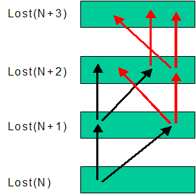
Fig. 5 - Move trees of two leapfrog cycles (black and red). Note that the red moves first catch up with the black (N+1 -> N+2), and then overtakes it by building on lost(N+2) created by itself, as well as the previous black leapfrog cycle.