Copolymer Composition Drift
a program for the Texas Instruments TI-83
and TI-84 (Plus) graphing calculators

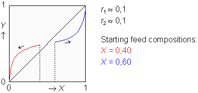
Summary

In a copolymerization process two (or more) monomer species M1 and M2 chemically react to form long-chained polymer molecules. During this process the ratio of the rates of reaction of the monomers M1 and M2 usually does not equal the ratio of the monomer concentrations in the solution. In other words, the composition of the copolymer chains produced in a very small time period usually differs from the monomer feed composition. For that reason the mole fractions of the momomers in the feed, X and (1–X), change as the copolymerization reaction proceeds. Consequently, the mole fractions of the momomers found in the polymer chains that are being produced, Y and (1–Y), change in course of time too.

Considering a reactive site at the end of the chain of a growing bipolymer, it could be a radical, or ionic species, or a coordination complex. Moreover, the active site can be either a remainder of monomer M1, or a remainder of M2, depending on which one of both monomers has been the latest to couple with the growing chain.
The relative preference of a specific reactive site for the monomers is given by the reactivity ratio r. Assuming only two different active extremities, it needs two reactivity ratios (r₁=k₁₁/k₁₂ and r₂=k₂₂/k₂₁) to enable calculating the instantaneous copolymer composition Y.

Using a rewritten version of the so-called "copolymer equation", which is applicable to many polymer systems, the program calculates the copolymer composition Y from a given X and reactivity ratios r₁ and r₂. To track the composition drift, it performs reiterative calculations in which the computed instantaneous copolymer composition Y is used to compute the next feed composition X.

The composition drift is visualized graphically by plotting the copolymer composition versus the feed composition. As the program runs, the compositions passed through are being represented as a lengthening curve, starting from the given X and ending as soon as the compositions no longer change.

To set an example: the program lets you track the composition drift coming up for discussion in problem 7 of the preliminary examination example Polymeren I. Here the initial value of the mole fraction in the feed X equals 0,50 and the reactivity ratios r₁ and r₂ are 0,0 and 1,0 respectively (see also the solution help at page 3 of the document). You can download Polymeren I from here.

While running the program, a composition drift curve is drawn. When the program execution is interrupted, you may press the ENTER key to continue and add another curve to the graph; or press the ON key to stop the program.
To acquire instantaneous feed and copolymer composition values from the displayed curves, use the four arrow keys after pressing the ON, 1 (Quit) and GRAPH keys.